Adaptive Projections

This page explains the options for adaptive convergence volumetric projections.

General Parameters

The following are important projection parameters in addition to the general Simulation ones:

proj_depth – Specifies the depth of the projection. If not explicitly set, it defaults to the value of image_width. [Units: cm]
proj_radius – Specifies the radius of the projection, which is half of the projection depth. This cannot be used if proj_depth is set. [Units: cm]
proj_radius_bbox – Specifies the radius of the projection relative to the bounding box. This cannot be used if proj_depth or proj_radius is set. [Default value: 0.]
adaptive – Enables the use of adaptive convergence in projections. When set to true, the projection algorithm uses a quadtree to automatically determine the optimal number of rays to use for each pixel. This is achieved by recursively subdividing the pixel until the error is below the specified tolerance. The error is estimated by comparing the results from a 4-point trapezoidal integration scheme to a second-order 9-point Simpson’s rule. [Default value: false]
pixel_rtol – Sets the relative tolerance per pixel when using adaptive convergence. It controls the maximum allowed error per pixel, allowing for accurate quantity-conserving projection images. [Default value: 0.01]
perspective – Enables the use of a perspective camera for rendering the projection. When set to true, the image rays will no longer be plane-parallel but will instead converge to a focal point. This provides a more realistic perception of distances as closer objects will appear larger than those that are farther away. [Default value: false]
stepback_factor – This determines the stepback distance for the projection, expressed as a factor relative to the image radius. It adjusts the viewpoint to conveniently capture the external perspective of an entire simulation volume, e.g. for large-scale cosmological boxes, as well as for creating animations of rotating galaxies. [Default value: 0.]
stepback_factor_bbox – Identical to the previous stepback_factor parameter for perspective cameras but is instead relative to the bounding box. [Default value: 0.]
proj_sphere – Enables the projection to be through a spherical volume. When set to true, the rays will be truncated to be within a sphere rather than a rectangular box. This is useful for creating rotation animations where features do not enter or exit the image due to being near the corners of the projected volume. [Default value: false]
proj_cylinder – Enables the projection to be through a cylindrical volume. Similar to the proj_sphere option, but the rays are truncated to be within a cylinder oriented along the camera north vector. This may be a more natural choice for rotation animations than using a sphere. [Default value: false]
override_volume – Allows for manually overridiong the projection volume normalization. Specifically, it allows for the pixel integration depths to vary according to the bounding box and projection shape volumes rather than using a constant value across the entire image based on the standard rectangular volume. [Default value: false]
shape_factor – Determines the extraction shape factor for the projection, expressed relative to the image radius. For example, this sets the radius of the sphere or cylinder for the proj_sphere and proj_cylinder options, respectively. [Default value: 0.]
shape_factor_bbox – Identical to the previous shape_factor parameter but is instead relative to the bounding box. [Default value: 0.]
fade_in_length – Specifies the characteristic position where the weights gradually increase from zero, setting the location of a Sigmoid filter within the projection volume. This is useful for minimizing abrupt entrance and exit effects when flying through a simulation volume, as well as maintaining the focus on the central object rather than the transition to the background. By default there is no fading. [Units: cm]
fade_in_length_bbox – Identical to the previous fade_in_length parameter but is instead relative to the bounding box. [Default value: 0.]
fade_in_width – Specifies the characteristic distance over which the weights gradually increase from zero, effectively controlling the smoothness of the projection integration edges setting the width of a Sigmoid filter within the projection volume. See the further comments regarding the fade_in_length parameter. [Units: cm]
fade_in_width_bbox – Identical to the previous fade_in_width parameter but is instead relative to the bounding box. [Default value: 0.]
fade_out_length – Identical to the fade_in_length parameter but for the exit side of the projection volume. [Units: cm]
fade_out_length_bbox – Identical to the previous fade_out_length parameter but is instead relative to the bounding box. [Default value: 0.]
fade_out_width – Identical to the fade_in_width parameter but for the exit side of the projection volume. [Units: cm]
fade_out_width_bbox – Identical to the previous fade_out_width parameter but is instead relative to the bounding box. [Default value: 0.]
field_weight_pairs – Accepts a list of projection field and weight pairs, which are used in the integration calculations. The field is the primary quantity of interest, e.g. density or temperature, while the weight biases the contribution based on a secondary quantity or normalization scheme. For example, providing [rho, avg] produces a volume-weighted density image along the line of sight, or \(\langle \rho \rangle_V \equiv \int \rho \, {\rm d}V / \int {\rm d}V\). Likewise, providing [T, mass] produces a mass-weighted temperature image, or \(\langle T \rangle_m \equiv \int T \rho \, {\rm d}V / \int \rho \, {\rm d}V\), and providing [SFR, sum] produces a total star formation rate image, or \(\sum {\rm SFR} \equiv \int \rho_{\rm SFR} \, {\rm d}V\), which is useful for conservative (non-density-like) fields. Finally, providing an arbitrary field and weight is equivalent to \(\langle f \rangle_w \equiv \int f w \, {\rm d}V / \int w \, {\rm d}V\) and will automatically produce the denominator image as well to allow reconstructing the numerator image later. The field names are case-sensitive and must match the simulation field names (see Gas Fields), however known aliases are also accepted, e.g. Density is equivalent to rho. The weights also allow aliases of Average, Mass, and Sum for avg, mass, and sum, respectively.
fields – Alternatively, a list of projection fields can be specified with volume-weighted integrations by default (avg). This is useful for simple projections where the weights are not needed. For example, [rho, T] is equivalent to [[rho, avg], [T, avg]].
weights – When the fields list is provided, a list of projection weights can be specified to override the avg default. This is useful if only the first weights differ from the default behavior. For example, [mass] is equivalent to [[rho, mass], [T, avg]] for the previous example.
kappa_field – Specifies the field name for the absorption opacity in the same sense as the radiative transfer equation. This is useful for emulating synthetic observations of emissivity- and obscuration-like fields, or for creating more intuitive images accounting for gas/dust column densities. The absorption opacity can be further modified via power-law modifications as specified below, such that the optical depth is \(\tau = \int \kappa_0 \kappa^\beta \rho^\gamma \, {\rm d}\ell\), where \(\kappa_0\) is an opacity scaling constant, \(\beta\) is an opacity exponent, \(\gamma\) is a density exponent, and \(\ell\) is the line-of-sight distance. By default the absorption opacity is disabled. [Default value: “”]
kappa_constant – Determines the absorption opacity scaling constant \(\kappa_0\) (see the kappa_field description). [Default value: 1.]
kappa_exponent – Determines the absorption opacity exponent \(\beta\) (see the kappa_field description). [Default value: 1.]
rho_exponent – Determines the absorption opacity density exponent \(\gamma\) (see the kappa_field description). [Default value: 1.]

These parameters should be defined in your configuration file, e.g., config-proj.yaml.

Quickstart Example

This section provides detailed explanations of setting up, running, and visualizing the results from the COLT projections module. For simplicity, our example is based on a dodecahedron shape, constructed from a Voronoi mesh with a single interior cell and 12 edge cells. The final image should look like the following:

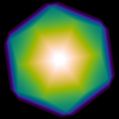
Projection Image — **Projection Example:** This image is a volume-weighted density image of a dodecahedron.

We suggest first setting up a directory structure as follows:

.proj-test            # Dodecahedron test directory
├── config-proj.yaml  # Configuration file
├── defines.yaml      # Compile time definitions
├── ics               # Initial conditions directory
│   ├── dodec.hdf5    # Initial conditions file (created by dodec.py)
│   └── dodec.py      # Initial conditions script (creates dodec.hdf5)
├── output            # Output directory (created by COLT)
│   └── proj.hdf5     # Projection output file (created by COLT)
├── plots             # Visualization directory
│   ├── dodec.png     # Final image (created by plot.py)
│   └── plot.py       # Visualization script (creates dodec.png)
└── run.sh            # Compilation and execution convenience script

The defines.yaml compile time definitions file should contain the following:

# Compile time definitions

GEOMETRY: voronoi  # Geometry type: slab, spherical, cartesian, octree, voronoi
# HAVE_CGAL: true    # Include the CGAL library (requires voronoi geometry)

CGAL is not strictly necessary for this example, but provides the general Voronoi mesh construction utilities COLT relies on. The initial conditions script ics/dodec.py should contain the following:

import numpy as np
import h5py

pc = 3.085677581467192e18  # 1 pc  = 3e18 cm
kpc = 1e3 * pc             # 1 kpc = 3e21 cm

# Create dodecahedron mesh
n_cells = 13  # Number of cells
C0 = 0.  # Center of dodecahedron
C1 = np.sqrt(2. - 2./np.sqrt(5.)) * kpc  # = 1.05146 kpc
C2 = np.sqrt(2. + 2./np.sqrt(5.)) * kpc  # = 1.70130 kpc
r = np.array([[ C0,  C0,  C0],  # Mesh generating points
    [ C1,  C0,  C2], [ C2,  C1,  C0], [ C0,  C2,  C1], [ C0,  C2, -C1],
    [ C1,  C0, -C2], [-C1,  C0,  C2], [ C0, -C2,  C1], [ C2, -C1,  C0],
    [ C0, -C2, -C1], [-C2,  C1,  C0], [-C1,  C0, -C2], [-C2, -C1,  C0]], dtype=np.float64)
one = np.ones(n_cells)  # Array of ones
cen = np.zeros(n_cells); cen[0] = 1.  # Center cell
with h5py.File(f'dodec.hdf5', 'w') as f:
    # Basic data (gas properties)
    f.attrs['n_cells'] = np.int32(n_cells)  # Number of cells
    f.attrs['r_box'] = np.float64(2.*kpc)  # Box radius [cm]
    f.create_dataset('r', data=r)  # Positions [cm]
    f['r'].attrs['units'] = b'cm'
    f.create_dataset('v', data=np.zeros_like(r))  # Velocities [cm/s]
    f['v'].attrs['units'] = b'cm/s'
    f.create_dataset('rho', data=cen)  # Density [g/cm^3]
    f['rho'].attrs['units'] = b'g/cm^3'
    f.create_dataset('T', data=one)  # Temperature [K]
    f['T'].attrs['units'] = b'K'
    # Voronoi mesh data (CGAL equivalent)
    f.attrs['n_circulators_tot'] = np.int32(60)  # Number of circulators
    f.attrs['n_edges'] = np.int32(12)  # Number of edge cells
    f.attrs['n_inner_edges'] = np.int32(1)  # Number of inner edge cells
    f.attrs['n_neighbors_tot'] = np.int32(84)  # Number of neighbors
    V0 = 10. * np.sqrt(130. - 58.*np.sqrt(5.)) * kpc**3  # = 5.55029 kpc^3
    f.create_dataset('V', data=V0*cen)  # Cell volumes [cm^3]
    f['V'].attrs['units'] = b'cm^3'
    ci = 60 * np.ones(85, dtype=np.int32)
    ci[:12] = [0, 5, 10, 15, 20, 25, 30, 35, 40, 45, 50, 55]
    cip = np.array([2, 8, 7, 6, 3, 3, 4, 5, 8, 1, 2, 4, 10, 6, 1, 10, 3, 2, 5,
        11, 9, 8, 2, 4, 11, 1, 3, 10, 12, 7, 6, 12, 9, 8, 1, 9, 7, 1, 2, 5, 11,
        12, 7, 8, 5, 12, 6, 3, 4, 11, 9, 12, 10, 4, 5, 6, 10, 11, 9, 7], dtype=np.int32)
    ni = np.array([0, 12, 18, 24, 30, 36, 42, 48, 54, 60, 66, 72, 78, 84], dtype=np.int32)
    nip = np.array([1, 2, 3, 4, 5, 6, 7, 8, 9, 10, 11, 12, 0, 2, 3, 6, 7, 8, 0,
        1, 3, 4, 5, 8, 0, 1, 2, 4, 6, 10, 0, 2, 3, 5, 10, 11, 0, 2, 4, 8, 9, 11,
        0, 1, 3, 7, 10, 12, 0, 1, 6, 8, 9, 12, 0, 1, 2, 5, 7, 9, 0, 5, 7, 8, 11,
        12, 0, 3, 4, 6, 11, 12, 0, 4, 5, 9, 10, 12, 0, 6, 7, 9, 10, 11], dtype=np.int32)
    f.create_dataset('circulator_indices', data=ci)  # Circulator indices
    f.create_dataset('circulator_indptr', data=cip)  # Circulator indptr
    f.create_dataset('edges', data=np.arange(1, 13, dtype=np.int32))  # Edge indices
    f.create_dataset('inner_edges', data=np.array([0], dtype=np.int32))  # Inner edges
    f.create_dataset('neighbor_indices', data=ni)  # Neighbor indices
    f.create_dataset('neighbor_indptr', data=nip)  # Neighbor indptr

This will create the ics/dodec.hdf5 file, which is specified as the initial conditions file in the configuration file config-proj.yaml. The HDF5 file stores the basic gas properties (density, temperature, etc.) as well as the Voronoi mesh connectivity data (edge cells, neighbors, circulators, etc.) that COLT uses for the projection.

The config-proj.yaml runtime configuration file should contain the following:

# COLT config file
--- !projections              # Ray-based projections module

init_file: ics/dodec.hdf5     # Initial conditions file
output_dir: output            # Output directory name
output_base: proj             # Output file base name

avoid_edges: false            # Avoid ray-tracing through edge cells
field_weight_pairs:
  - [rho, avg]                # Pairs of fields and weights

# Camera Information
image_radius_bbox: 0.6        # Image radius relative to the bounding box
proj_radius_bbox: 0.6         # Projection radius relative to the bounding box
n_pixels: 400                 # Number of image pixels (resolution)
camera: [1,1,1]               # Camera orientation

This supplies the initial conditions file, output directory, and output file base name. The avoid_edges option is set to false to allow the rays to pass through the edge cells without artificial termination. The field_weight_pairs option specifies the density field and volume-weighted integration. The image_radius_bbox and proj_radius_bbox options specify the image size and projection depth relative to the bounding box, respectively. The n_pixels option specifies the number of image pixels, and the camera option specifies the viewing direction.

At this point COLT can be compiled and executed, which will create the output/proj.hdf5 file that stores the raw projection data. To visualize the results, we provide a plots/plot.py script that creates the final image and should contain the following:

import numpy as np
import h5py, cmasher
import matplotlib.pyplot as plt
from matplotlib.colors import Normalize

# Plot dodecahedron image
with h5py.File(f'../output/proj.hdf5', 'r') as f:
    Z = f['proj_rho_avg'][0]; Z /= np.max(Z)
    R = f.attrs['image_radius']
    extent = [-R, R, -R, R]
fig = plt.figure(figsize=(4., 4.))
ax = plt.axes([0, 0, 1, 1])
ax.imshow(Z.T, origin='lower', extent=extent, cmap='cmr.rainforest', aspect='equal',
            interpolation='bicubic', norm=Normalize(vmin=0., vmax=1.))
ax.set_axis_off()
fig.savefig('dodec.png', bbox_inches='tight', pad_inches=0., dpi=100)

For convenience, we provide a full bash script for generating initial conditions, compiling, running, and plotting the results for the dodecahedron example. This should be run within the top proj-test directory with bash run.sh and contains the following:

#!/bin/bash

# Generate initial conditions
cd ics  # Navigate to the ics directory
python3 dodec.py  # Create the initial conditions file
cd ..  # Navigate back to the test directory

# Compile COLT
code_path=$(realpath "/path/to/colt")  # Set path to COLT source code
run_path=$(realpath ".")  # Set path to COLT test directory
opts="DEFS=$run_path/defines.yaml BUILD=$run_path/build EXE=$run_path/colt"
make clean_exe $opts -C $code_path
make -j $opts -C $code_path

# Run COLT
export OMP_NUM_THREADS=16
mpirun -n 1 ./colt config-proj.yaml

# Plot the results
cd plots  # Navigate to the plots directory
python3 plot.py  # Create the plot
cd ..  # Navigate back to the test directory

Note that the OMP_NUM_THREADS environment variable is set to enable OpenMP parallelism for the projection algorithm to process multiple image pixels at a time. When making projections of large simulations for multiple cameras, it is recommended to also use MPI parallelism to process multiple cameras at a time, which can be achieved with mpirun -n [n_tasks] ./colt config-proj.yaml. We recommend using one MPI task per node (at most the number of cameras) and one OpenMP thread per core for optimal performance.