Projections and Visualization
The projections module traces rays through the simulation volume and reduces gas or star fields onto camera images. This page describes how to choose the line-of-sight extent, ray geometry, integration method, volume normalization, and projected quantities. General camera placement, orientation, and image-plane sampling are documented under Simulation.
General Parameters
The runtime parameters are grouped below by the part of the projection that they control.
Projection extent
The image dimensions set the projected area in the camera plane. The following parameters independently set the integration extent along the line of sight. proj_depth, proj_depth_cMpc, proj_radius, proj_radius_bbox, and proj_radius_Rvir are mutually exclusive.
proj_depth– Sets the full line-of-sight integration depth. If no depth or radius is configured, COLT uses the mean of the two image widths. [Default value: mean image width | Units: cm | Valid range: proj_depth >= 0]proj_depth_cMpc– Sets the full line-of-sight integration depth in comoving megaparsecs. COLT converts this value to a physical depth using the simulation redshift. [Optional | Units: cMpc | Valid range: proj_depth_cMpc >= 0]proj_radius– Sets the projection half-depth, so the full line-of-sight depth is2 * proj_radius. [Optional | Units: cm | Valid range: proj_radius >= 0]proj_radius_bbox– Sets the projection half-depth relative to the shortest distance fromcamera_centerto a bounding-box face. For example,proj_radius_bbox: 1makes the half-depth equal to that minimum distance. [Optional | Units: bounding-box distance | Valid range: proj_radius_bbox >= 0]proj_radius_Rvir– Sets the projection half-depth in units of the selected halo virial radius \(R_{\rm vir}\). [Requires a selected halo | Optional | Units: Rvir | Valid range: proj_radius_Rvir >= 0]n_slices– Divides the projection depth into this many line-of-sight slabs and writes a separate result for each slab. Histogram projections require the default single slice. [Default value: 1 | Valid range: n_slices > 0]
Integration and camera modes
adaptive– Enables adaptive spatial integration in the image plane. A quadtree recursively subdivides each pixel and compares four-point trapezoidal integration with nine-point Simpson integration. Refinement stops when the estimated relative error satisfiespixel_rtol. Adaptive projections are not currently compatible with perspective cameras, spherical or cylindrical clipping, line-of-sight or radial fading, orkappa_field. [Default value: false]pixel_rtol– Sets the target relative integration tolerance for each adaptively refined pixel. Smaller values generally increase accuracy by tracing more rays, at greater computational cost. This parameter is read only whenadaptiveis true. [Requires adaptive | Default value: 0.01 | Valid range: finite and > 0]perspective– Replaces the default plane-parallel rays with rays that converge on a focal point. Objects closer to the observer therefore appear larger than more distant objects. Perspective and monoscopic modes cannot be enabled together, and adaptive perspective projections are not currently implemented. [Default value: false]monoscopic– Produces a 360-degree equirectangular image for virtual-reality or panoramic viewing. COLT enforces the required 2:1 aspect ratio by settingnx_pixelsto2 * ny_pixels. Slit, cube, radial-image, and radial-cube outputs are disabled because their geometries are incompatible with this mode. [Default value: false]stepback_factor– Moves the observer away fromcamera_centerin units of the projection radius. For a perspective camera, the focal point is displaced bystepback_factor * proj_radius. For a monoscopic camera, ray origins lie at(1 + stepback_factor) * proj_radius. Increasing the value is useful when framing external views of a simulation volume or making rotating-camera animations. [Default value: 0.]stepback_factor_bbox– Sets the observer displacement relative to the shortest distance fromcamera_centerto a bounding-box face. It is converted tostepback_factorusingproj_radius_bbox. [Requires proj_radius_bbox | Optional | Units: bounding-box distance]stepback_factor_Rvir– Sets the observer displacement in units of the selected halo virial radius. It is converted tostepback_factorusingproj_radius_Rvir. [Requires proj_radius_Rvir and a selected halo | Optional | Units: Rvir]
Clipping and normalization
proj_sphere– Clips each ray to a sphere centered oncamera_centerinstead of integrating through the standard rectangular volume. A spherical boundary prevents material near the corners of a box-shaped volume from entering and leaving the frame during camera rotations. [Default value: false]proj_cylinder– Clips each ray to a cylinder centered oncamera_centerand oriented alongcamera_north. For some rotating views, this retains more of the target along the rotation axis than spherical clipping. [Default value: false]shape_factor– Sets the clipping sphere or cylinder radius in units ofproj_radius. It is used only whenproj_sphereorproj_cylinderis enabled; a value of1makes the clipping radius equal to the projection half-depth. [Default value: 1.]shape_factor_bbox– Sets the clipping radius relative to the shortest distance fromcamera_centerto a bounding-box face. It is converted toshape_factorusingproj_radius_bbox. [Requires proj_radius_bbox and a clipping shape | Optional | Units: bounding-box distance]shape_factor_Rvir– Sets the clipping radius in units of the selected halo virial radius. It is converted toshape_factorusingproj_radius_Rvir. [Requires proj_radius_Rvir, a selected halo, and a clipping shape | Optional | Units: Rvir]override_volume– Uses the configured slice or projection depth when normalizing each pixel, rather than the ray’s actual path length after bounding-box or shape clipping. Enable this when output values should share a constant reference volume across the image. Leave it disabled when averages should be normalized by the material depth actually traversed by each ray. [Default value: false]
Distance weighting
The fade parameters multiply each gas-cell or star contribution by smooth logistic weights between zero and one. Line-of-sight fades select a depth interval along the viewing direction; radial fades select a spherical distance interval around camera_center. Either family may define an inner fade, an outer fade, or both. Distance weighting is not currently compatible with adaptive integration.
fade_in_length– Sets the midpoint of the line-of-sight entrance transition. Contributions before this depth are suppressed, while contributions after it are retained. Omitting allfade_in_length*parameters disables the entrance fade. [Optional | Units: cm]fade_in_width– Controls how gradually the entrance weight changes aroundfade_in_length. A smaller positive width produces a sharper transition. [Used with fade_in_length | Units: cm | Valid range: fade_in_width > 0]fade_out_length– Sets the midpoint of the line-of-sight exit transition. Contributions before this depth are retained, while contributions after it are suppressed. Omitting allfade_out_length*parameters disables the exit fade. [Optional | Units: cm]fade_out_width– Controls how gradually the exit weight changes aroundfade_out_length. A smaller positive width produces a sharper transition. [Used with fade_out_length | Units: cm | Valid range: fade_out_width > 0]
Note
Each line-of-sight parameter also accepts a *_bbox form (fade_in_length_bbox, fade_in_width_bbox, fade_out_length_bbox, and fade_out_width_bbox), measured relative to the shortest distance from camera_center to a bounding-box face. The corresponding *_Rvir forms are measured in units of the selected halo virial radius.
radial_fade_in_length– Sets the midpoint of the inner radial transition aroundcamera_center. Contributions at smaller radii are suppressed, while contributions beyond this radius are retained. Omitting allradial_fade_in_length*parameters disables the inner radial fade. [Optional | Units: cm]radial_fade_in_width– Controls how gradually the inner radial weight changes aroundradial_fade_in_length. [Used with radial_fade_in_length | Units: cm | Valid range: radial_fade_in_width > 0]radial_fade_out_length– Sets the midpoint of the outer radial transition aroundcamera_center. Contributions at smaller radii are retained, while contributions beyond this radius are suppressed. Omitting allradial_fade_out_length*parameters disables the outer radial fade. [Optional | Units: cm]radial_fade_out_width– Controls how gradually the outer radial weight changes aroundradial_fade_out_length. [Used with radial_fade_out_length | Units: cm | Valid range: radial_fade_out_width > 0]
Note
Each radial parameter also accepts a *_bbox form (for example, radial_fade_in_length_bbox) and a *_Rvir form (for example, radial_fade_in_length_Rvir). These use the same bounding-box-distance and virial-radius conventions as the line-of-sight variants.
Projected fields and opacity
field_weight_pairs– Selects gas fields and their integration weights as a YAML list of[field, weight]pairs. Field names are case-sensitive and must match Gas Fields, although documented aliases such asDensityandrhoare equivalent. Weight names accept the short formsavg,mass, andsumor the aliasesAverage,Mass, andSum.Example field and weight combinations Configuration
Result
Interpretation
[rho, avg]\(\langle \rho \rangle_V = \int \rho \, {\rm d}V / \int {\rm d}V\)
Volume-weighted mean density along each ray.
[T, mass]\(\langle T \rangle_m = \int T\rho \, {\rm d}V / \int \rho \, {\rm d}V\)
Mass-weighted mean temperature.
[SFR, sum]\(\int \rho_{\rm SFR} \, {\rm d}V\)
Conserved total for a non-density-like field.
[f, w]\(\langle f \rangle_w = \int fw \, {\rm d}V / \int w \, {\rm d}V\)
Mean of
fweighted by an arbitrary fieldw.For an arbitrary field weight, COLT also writes the denominator projection. This makes it possible to reconstruct the unnormalized numerator after the run.
fields– Provides a shorter form when the field and weight pairs do not need to be written explicitly. Each listed field receives theavgweight unlessweightssupplies a corresponding override. For example,fields: [rho, T]is equivalent tofield_weight_pairs: [[rho, avg], [T, avg]]. [Default value: [Density]]weights– Overrides weights positionally for entries infields. Missing entries are filled withavgand extra entries are ignored. Withfields: [rho, T], for example,weights: [mass]is equivalent tofield_weight_pairs: [[rho, mass], [T, avg]].kappa_field– Names the gas field used as an absorption-opacity proxy. When configured, each projected field is attenuated along the ray according to \(\tau = \int \kappa_0 \kappa^\beta \rho^\gamma \, {\rm d}\ell\), where \(\kappa\) is the selected field, \(\rho\) is the gas density, and \(\ell\) is line-of-sight distance. This supports synthetic observations that combine emissivity-like fields with gas or dust obscuration. Opacity is disabled when the name is empty and is not currently compatible with adaptive integration. [Default value: “”]kappa_constant– Sets the positive opacity scaling coefficient \(\kappa_0\) in the equation above. [Requires kappa_field | Default value: 1. | Valid range: kappa_constant > 0]kappa_exponent– Sets the exponent \(\beta\) applied to the selected opacity field. [Requires kappa_field | Default value: 1.]rho_exponent– Sets the exponent \(\gamma\) applied to gas density in the opacity calculation. [Requires kappa_field | Default value: 1.]star_field_weight_pairs– Selects star fields and weights as[field, weight]pairs. Unlike gas projections, these are discrete sums over stars assigned to each pixel. For example,[Z, m]produces the mass-weighted stellar metallicity \(\langle Z \rangle_m = \sum mZ / \sum m\). Names are case-sensitive and must match Star Fields, with aliases such asStellarMass,m, andm_staraccepted where documented. The weights also acceptAverageandSumas aliases foravgandsum.
Define these parameters in the projections-module YAML configuration, such as the config-proj.yaml file in the example below.
Quickstart Example
This quickstart shows how to set up, run, and visualize a COLT projection. The example uses a dodecahedron represented by a Voronoi mesh with one interior cell and 12 surrounding edge cells. The final image should look like this:
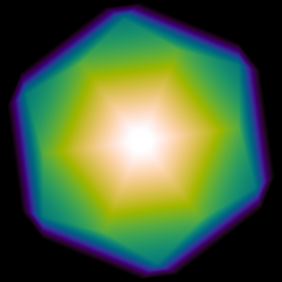
Projection Example: This image is a volume-weighted density image of a dodecahedron.
Create the following directory structure:
proj-test/            # Dodecahedron test directory
├── config-proj.yaml  # Configuration file
├── defines.yaml      # Compile-time definitions
├── ics               # Initial conditions directory
│   ├── dodec.hdf5    # Initial conditions file (created by dodec.py)
│   └── dodec.py      # Initial conditions script (creates dodec.hdf5)
├── output            # Output directory (created by COLT)
│   └── proj.hdf5     # Projection output file (created by COLT)
├── plots             # Visualization directory
│   ├── dodec.png     # Final image (created by plot.py)
│   └── plot.py       # Visualization script (creates dodec.png)
└── run.sh            # Compilation and execution convenience script
The defines.yaml compile-time definitions file should contain the following:
# Compile-time definitions

GEOMETRY: voronoi  # Geometry type: slab, spherical, cylindrical, cartesian, block_cartesian, octree, voronoi
# HAVE_CGAL: true  # Include the CGAL library (requires voronoi geometry)
CGAL is not strictly necessary for this example, but provides the general Voronoi mesh construction utilities COLT relies on. The initial conditions script ics/dodec.py should contain the following:
import h5py
import numpy as np

kpc = 3.085677581467192e21  # 1 kpc = 3e21 cm

# Create dodecahedron mesh
n_cells = 13  # Number of cells
c0 = 0.  # Center of dodecahedron
c1 = np.sqrt(2. - 2./np.sqrt(5.)) * kpc  # = 1.05146 kpc
c2 = np.sqrt(2. + 2./np.sqrt(5.)) * kpc  # = 1.70130 kpc
r = np.array([[ c0,  c0,  c0],  # Mesh-generating points
    [ c1,  c0,  c2], [ c2,  c1,  c0], [ c0,  c2,  c1], [ c0,  c2, -c1],
    [ c1,  c0, -c2], [-c1,  c0,  c2], [ c0, -c2,  c1], [ c2, -c1,  c0],
    [ c0, -c2, -c1], [-c2,  c1,  c0], [-c1,  c0, -c2], [-c2, -c1,  c0]], dtype=np.float64)
one = np.ones(n_cells)  # Array of ones
center = np.zeros(n_cells)
center[0] = 1.  # Select the center cell
with h5py.File('dodec.hdf5', 'w') as f:
    # Basic data (gas properties)
    f.attrs['n_cells'] = np.int32(n_cells)  # Number of cells
    f.attrs['r_box'] = np.float64(2.*kpc)  # Box radius [cm]
    f.create_dataset('r', data=r)  # Positions [cm]
    f['r'].attrs['units'] = b'cm'
    f.create_dataset('v', data=np.zeros_like(r))  # Velocities [cm/s]
    f['v'].attrs['units'] = b'cm/s'
    f.create_dataset('rho', data=center)  # Density [g/cm^3]
    f['rho'].attrs['units'] = b'g/cm^3'
    f.create_dataset('T', data=one)  # Temperature [K]
    f['T'].attrs['units'] = b'K'
    # Voronoi mesh data (CGAL equivalent)
    f.attrs['n_circulators_tot'] = np.int32(60)  # Number of circulators
    f.attrs['n_edges'] = np.int32(12)  # Number of edge cells
    f.attrs['n_inner_edges'] = np.int32(1)  # Number of inner edge cells
    f.attrs['n_neighbors_tot'] = np.int32(84)  # Number of neighbors
    central_volume = 10. * np.sqrt(130. - 58.*np.sqrt(5.)) * kpc**3
    f.create_dataset('V', data=central_volume*center)  # Cell volumes [cm^3]
    f['V'].attrs['units'] = b'cm^3'
    ci = 60 * np.ones(85, dtype=np.int32)
    ci[:12] = [0, 5, 10, 15, 20, 25, 30, 35, 40, 45, 50, 55]
    cip = np.array([2, 8, 7, 6, 3, 3, 4, 5, 8, 1, 2, 4, 10, 6, 1, 10, 3, 2, 5,
        11, 9, 8, 2, 4, 11, 1, 3, 10, 12, 7, 6, 12, 9, 8, 1, 9, 7, 1, 2, 5, 11,
        12, 7, 8, 5, 12, 6, 3, 4, 11, 9, 12, 10, 4, 5, 6, 10, 11, 9, 7], dtype=np.int32)
    ni = np.array([0, 12, 18, 24, 30, 36, 42, 48, 54, 60, 66, 72, 78, 84], dtype=np.int32)
    nip = np.array([1, 2, 3, 4, 5, 6, 7, 8, 9, 10, 11, 12, 0, 2, 3, 6, 7, 8, 0,
        1, 3, 4, 5, 8, 0, 1, 2, 4, 6, 10, 0, 2, 3, 5, 10, 11, 0, 2, 4, 8, 9, 11,
        0, 1, 3, 7, 10, 12, 0, 1, 6, 8, 9, 12, 0, 1, 2, 5, 7, 9, 0, 5, 7, 8, 11,
        12, 0, 3, 4, 6, 11, 12, 0, 4, 5, 9, 10, 12, 0, 6, 7, 9, 10, 11], dtype=np.int32)
    f.create_dataset('circulator_indices', data=ci)  # Cumulative n_circulators count
    f.create_dataset('circulator_indptr', data=cip)  # Circulator cell indices (flat)
    f.create_dataset('edges', data=np.arange(1, 13, dtype=np.int32))  # Edge indices
    f.create_dataset('inner_edges', data=np.array([0], dtype=np.int32))  # Inner edges
    f.create_dataset('neighbor_indices', data=ni)  # Cumulative n_neighbors count
    f.create_dataset('neighbor_indptr', data=nip)  # Neighbor cell indices (flat)
This creates ics/dodec.hdf5, the initial conditions file named by config-proj.yaml. It contains the basic gas properties and the Voronoi connectivity data that COLT needs to traverse edge cells, neighbors, and circulators.
The config-proj.yaml runtime configuration file should contain the following:
# COLT config file
--- !projections              # Ray-based projections module

init_file: ics/dodec.hdf5     # Initial conditions file
output_dir: output            # Output directory name
output_base: proj             # Output file base name

avoid_edges: false            # Avoid ray-tracing through edge cells
field_weight_pairs:
  - [rho, avg]                # Pairs of fields and weights

# Camera setup
image_radius_bbox: 0.6        # Image radius relative to the bounding box
proj_radius_bbox: 0.6         # Projection radius relative to the bounding box
n_pixels: 400                 # Number of image pixels (resolution)
camera: [1, 1, 1]             # Camera orientation
This supplies the initial conditions file, output directory, and output file base name. The avoid_edges option is set to false to allow the rays to pass through the edge cells without artificial termination. The field_weight_pairs option specifies the density field and volume-weighted integration. The image_radius_bbox and proj_radius_bbox options specify the image size and projection depth relative to the bounding box, respectively. The n_pixels option specifies the number of image pixels, and the camera option specifies the viewing direction.
At this point COLT can be compiled and executed, which will create the output/proj.hdf5 file that stores the raw projection data. To visualize the results, we provide a plots/plot.py script that creates the final image and should contain the following:
import cmasher
import h5py
import matplotlib.pyplot as plt
import numpy as np
from matplotlib.colors import Normalize

# Plot dodecahedron image
with h5py.File('../output/proj.hdf5', 'r') as f:
    image = f['proj_rho_avg'][0]
    image /= np.max(image)
    image_radius = f.attrs['image_radius']
    extent = [-image_radius, image_radius, -image_radius, image_radius]
fig = plt.figure(figsize=(4., 4.))
ax = plt.axes([0, 0, 1, 1])
ax.imshow(image.T, origin='lower', extent=extent, cmap='cmr.rainforest', aspect='equal',
            interpolation='bicubic', norm=Normalize(vmin=0., vmax=1.))
ax.set_axis_off()
fig.savefig('dodec.png', bbox_inches='tight', pad_inches=0., dpi=100)
For convenience, we provide a full bash script for generating initial conditions, compiling, running, and plotting the results for the dodecahedron example. This should be run within the top proj-test directory with bash run.sh and contains the following:
#!/usr/bin/env bash
set -euo pipefail

# Generate initial conditions
(cd ics && python3 dodec.py)

# Set the path to the COLT source code
colt_source="/path/to/colt"
example_dir="$(pwd)"  # Current example directory

# Keep build products inside the example directory
make -C "${colt_source}" \
    DEFS="${example_dir}/defines.yaml" \
    BUILD="${example_dir}/build" \
    EXE="${example_dir}/colt" -j

# Run COLT
export OMP_NUM_THREADS=16
./colt config-proj.yaml

# Plot the results
(cd plots && python3 plot.py)
The OMP_NUM_THREADS environment variable enables OpenMP parallelism over image pixels. Large runs with multiple cameras can also use MPI to distribute cameras, for example mpirun -n [n_tasks] ./colt config-proj.yaml. We recommend at most one MPI task per camera, usually one task per node, and one OpenMP thread per core.